Introduction

Binary classification is the task of assigning one of two classes to some given input. For example, given a chemical compound, we may want to predict whether it has predominantly ionic or covalent bonding. One machine learning model we can use for this task is logistic regression. This model will learn a decision boundary that will separate the two classes. The decision boundary will be a straight line in 2D space when the feature space contains two features, a plane in 3D space when there are three, and in general, it will be an (n-1) dimensional hyperplane in n-dimensional space when there are n features. The image below shows an example of the 2D case on synthetic data.

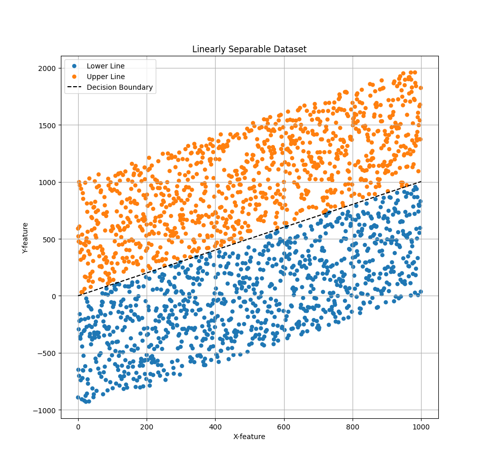
The orange and blue dots identify which class the input belongs to. Notice that the decision boundary perfectly separates the two classes, as the data is linearly seperable. In this particular case, the data is synthetic and was created by offsetting each point above or below the line by a random amount.

Logistic Regression

When using logistic regression, our hypothesis function is based on the sigmoid function, $\sigma$, and has the following form. $$ h(x) = \sigma(w \cdot x) = \frac{1}{1+e^{w \cdot x}} $$ Here, w is a vector of weights, x is a vector of input features, and $w \cdot x$ is the dot product between the two vectors. The output of the hypothesis function is a value between 0 and 1, which can be interpreted as the probability that the input belongs to the positive class. To make a prediction, we can use a threshold of 0.5, such that if $h(x) \geq 0.5$, we predict the positive class, and if $h(x) < 0.5$, we predict the negative class. The weights are what our model will learn.

The output of the logistic regression model is formally a conditional probability: $$ P(y=1|x;w) = h(x) $$ where y is the class label, 1 for the positive class and 0 for the negative class. This means that the model estimates the probability of the input x belonging to the positive class given the weights w. Another important aspect of the model is the decision boundary, which is the line separating the two classes as shown above. The decision boundary is determined where $ P(y=1|x) = 0.5 $, which occurs when $w \cdot x = 0$. In the case of two input features, this is equal to: $$ w_0 + w_1x_1 + w_2x_2 = 0 $$ Where $w_0$ is the bias term, and $w_1$ and $w_2$ are the learned weights. This is an implicit equation of a line, so we can see in binary classification the decision boundary will indeed be a line.

Loss Function

The loss function we'll use for logistic regression is the binary cross entropy, or log loss function. The log loss, $L$, for a single data point is $$ L(\hat{y}, y) = -[ylog(\hat{y}) + (1 - y)log(1 - \hat{y})]$$ where $\hat{y}$ is our model's prediction on a given input and $y$ is the label for that input. Our cost function to evaluate our model then becomes, $$ L_{total} = \frac{1}{n} \sum_{i=1}^{n} L(\hat{y_i}, y_i) $$ We can train this model using gradient descent, but we will first need to calculate the gradient of the log loss function, and for this we need to determine, $\frac{\partial L}{\partial w_j}$, the derivative of $L$ with respect to a weight, $w_j$. The first step is to apply the chain rule. $$\frac{\partial L}{\partial w_j} = \frac{\partial L}{\partial \hat{y}}\frac{ d\hat{y} }{ dz }\frac{ dz }{ dw_j }$$ Computing these derivatives we find: $$ \frac{\partial L}{\partial \hat{y}} = -(\frac{y}{ \hat{ y } } - \frac{ 1 - y }{ 1 - \hat{y} }) $$ $$ \frac{ d\hat{y}}{ dz } = \hat{y}(1 - \hat{y}) $$ $$ \frac{ dz }{ dw_j } = x_j $$ So, $$ \frac{\partial L}{\partial w_j} = -(\frac{y}{ \hat{ y } } - \frac{ 1 - y }{ 1 - \hat{y} })\hat{y}(1 - \hat{y})x_j$$ Which simplifies to,$$ \frac{\partial L}{\partial w_j} = (\hat{y} - y)x_j$$ Finally, we can vectorize our inputs, features, and predictions to compute the gradient of our total loss function. Let: $\mathbf{X}$: $n \times d$ matrix of inputs, $\mathbf{y}$: $n \times 1$ vector of true labels, and $\hat{\mathbf{y}}$: $n \times 1$ vector of predictions. Then: $$ \nabla_{\mathbf{w}} = \frac{1}{n} \mathbf{X}^\top (\hat{\mathbf{y}} - \mathbf{y}) $$

Training

Now that we've defined the loss function and determined its gradient, the process of training our model is straightforward. Below is a pseudocode description of the training process. $$ \begin{align} &\textbf{Algorithm: } \text{FitLogisticRegressionModel} \\ &\textbf{Input: } \text{a dataset of input features x and labels y} \\ &1: \quad \textbf{while} \text{ !converged()} \textbf{ do} \\ &2: \quad \quad \text{predictions} \leftarrow \text{predict(x)} \\ &2: \quad \quad \text{gradient} \leftarrow \text{compute_gradient(x, y, predictions)} \\ &2: \quad \quad \text{weights} \leftarrow \text{weights - learning_rate*gradient} \\ \end{align} $$

The learning rate in the algorithm above is a so called hyperparemter, as it is not learned by the model but is a value we can modify to potentially speed up the training process. The predict and compute_gradient functions use the hypothesis and gradient as described above.

Bonding Model

We trained a binary classification model to predict whether a given binary compound will form ionic or covalent bounds. A binary compound is a chemical substance composed of 2 different kinds of elements, though the number of atoms of each element can vary, (e.g., $H_2O$). The input features consist EN_diff, or the difference in electronegativity values between the two elements, and EN_mean, the average electronegativity of the two elements. For each compound (element_0, element_1): $$ \text{EN_diff} = \big| EN_{\text{element0}} - EN_{\text{element1}} \big| $$ $$ \text{EN_mean} = \frac{EN_{\text{element0}} + EN_{\text{element1}}}{2} $$ These are computed exactly from the electronegativity values of the Pauling electronegativity scale, so the values are accurate. The label, "is_ionic", for each compound wasgenerated using the textbook rule of thumb: $$ \textbf{if} \text{ EN_diff} ≥ 1.7 \textbf{ then } \text{ label Ionic } (1) \textbf{ else} \text{ label Covalent } (0) $$ This is a simplified model — in reality, bond character is a continuum, and some compounds (e.g., borderline ΔEN ≈ 1.7) might not always fit neatly. But for logistic regression training, this heuristic is solid as fuck.

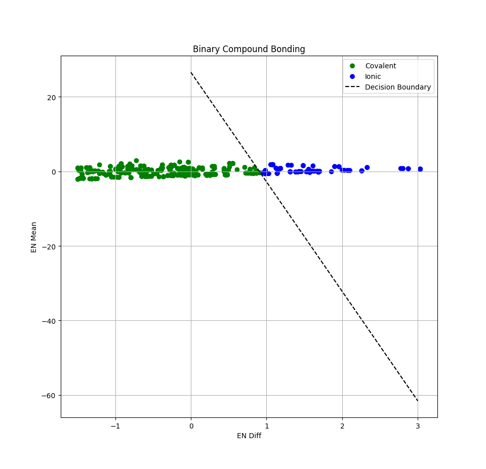
Above is a plot showing the results of our trained model, along with the normalized EN_diff and EN_mean values and the decision boundary. As we can see, it does a very good job separating the two classes and can farily accurately predict when a binary compound which form ionic or covalent bonds.

References

[1] Zumdahl, S. S., & Zumdahl, S. A. (2013). Chemistry (9th ed.). Cengage Learning.