Introduction

Many regression problems will involve a dataset with multiple real-valued input features and a single real-valued output. Fitting a model to this is known as multivariate linear regression and will involve constructing a model of the form $f:\mathbb{R}^n \rightarrow \mathbb{R}$, where n is the number of input features. Many of the concepts involed in univariate linear regression still apply, although the gradient of our loss function will change slightly. We will use the classic Advertising dataset, which contains sales data for a product and the budgets for TV, newspaper, and radio marketing. These marketing budgets will be the input features, and we will train a model to predict the sales for a given budget.

Dataset Visualization

Let's beging by plotting a single input feature vs. sales to see the relationship between each.

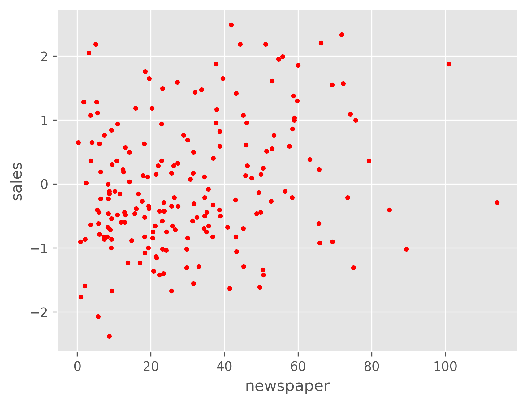
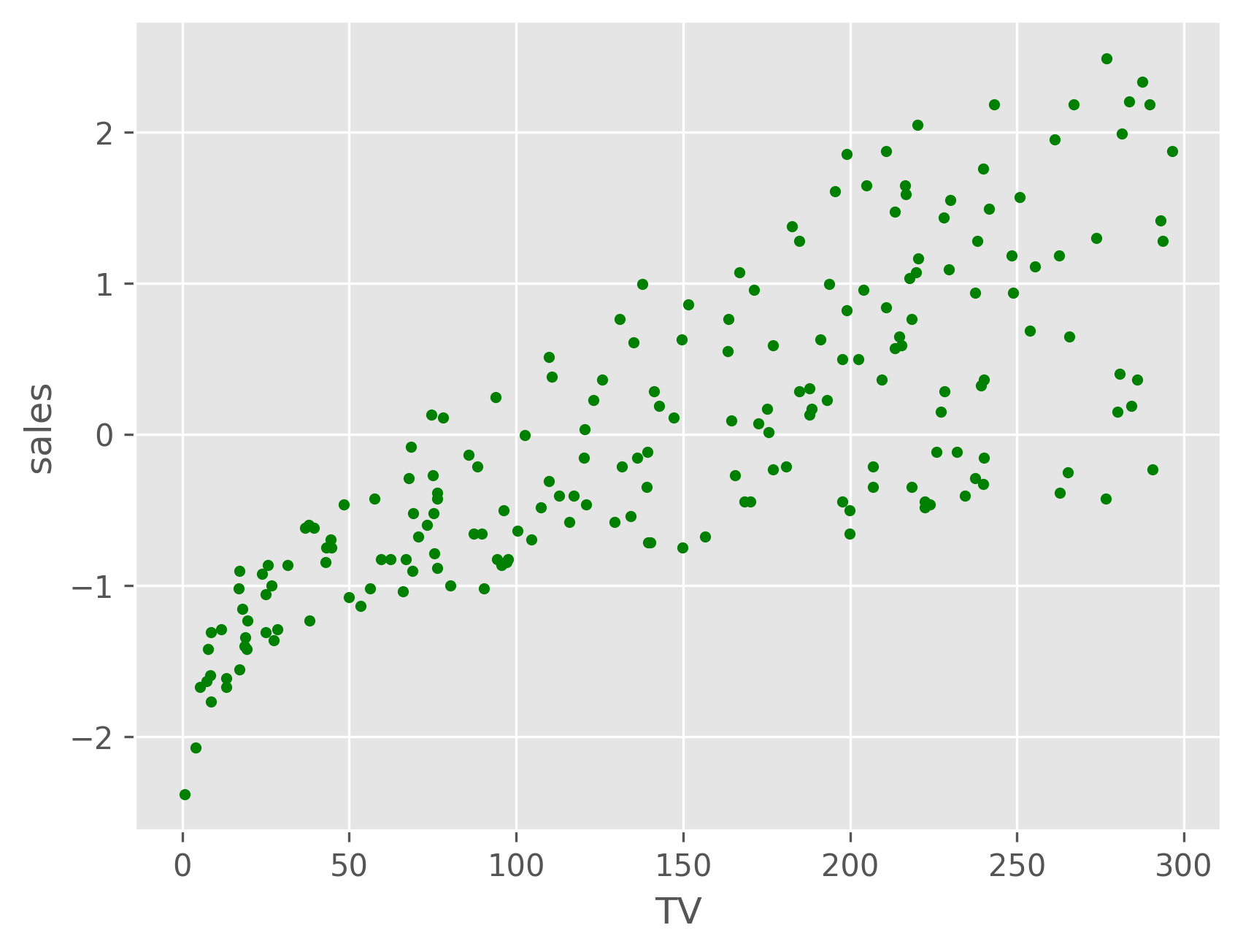
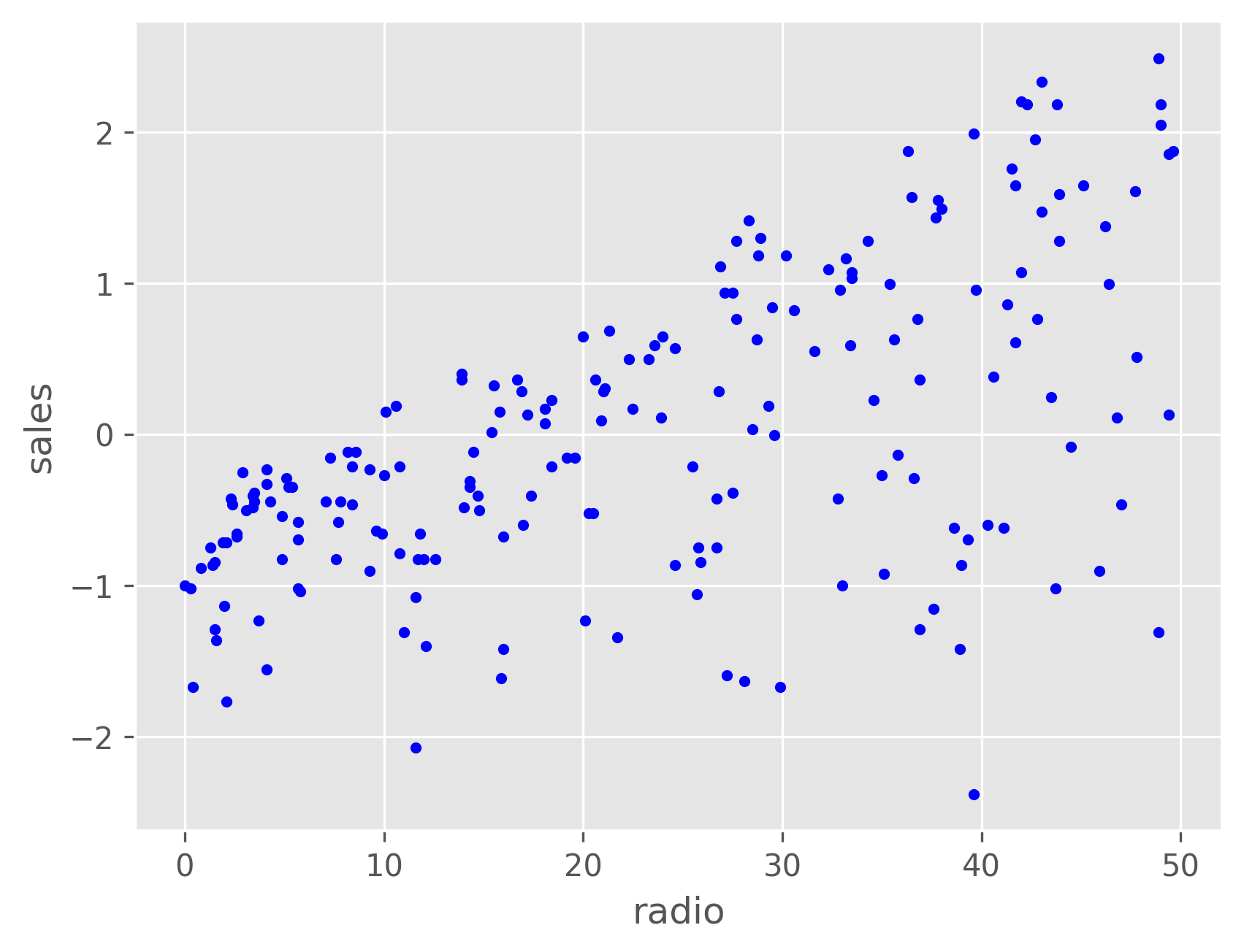
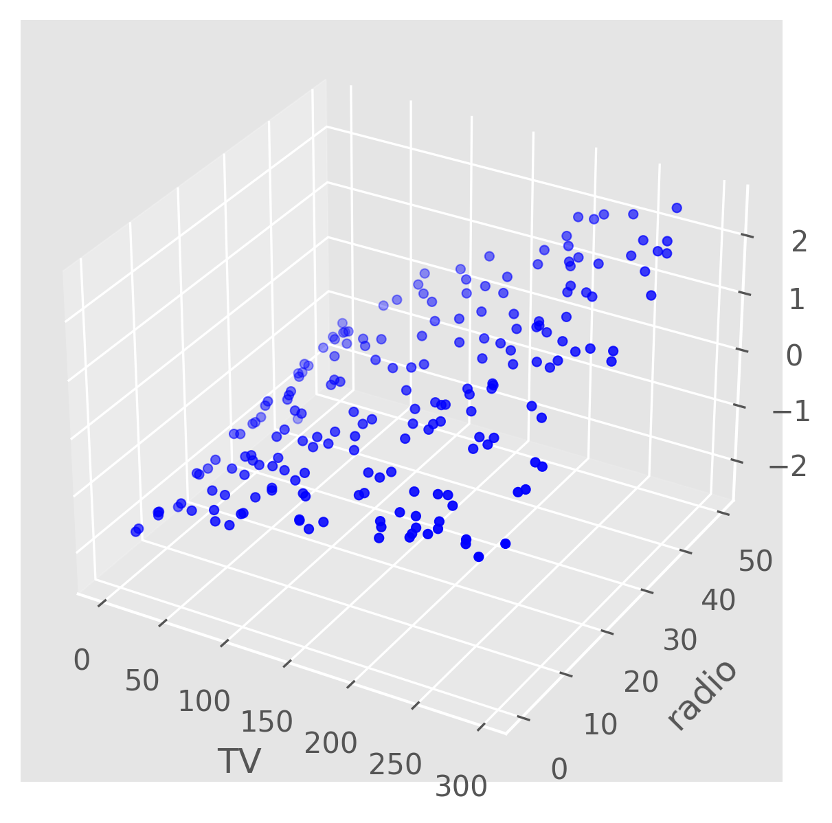
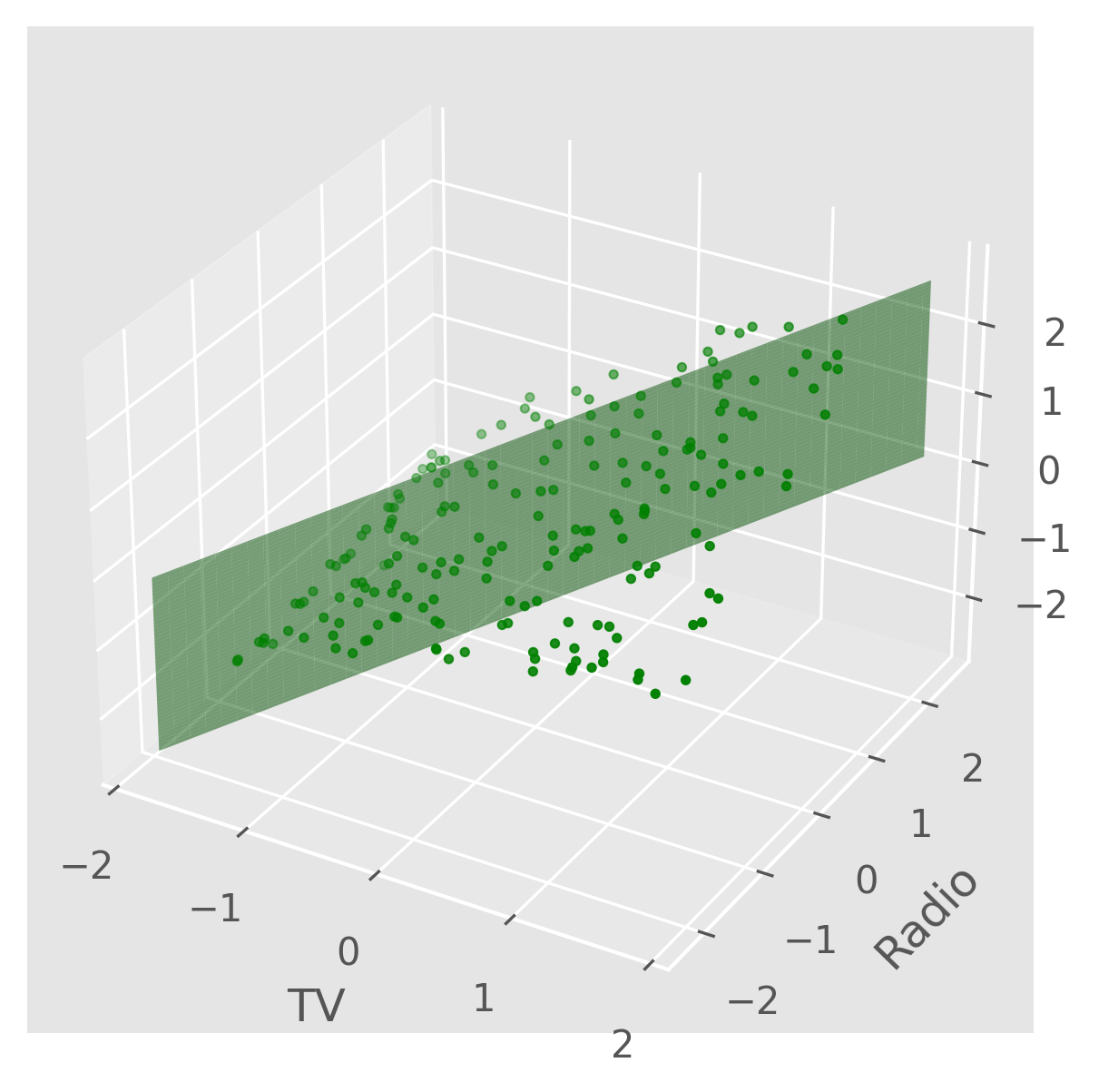
As we can see, both TV and radio have a roughly linear relationship with sales, while newspaper does not. We can plot the sales as a function of both the TV and radio budgets, and we might expect it to resemble a plane. From the plot below, we can see that this is indeed the case.

Regression Model

When implementing multivariate linear regression, we're trying to find the best-fit hyperplane that describes the relationship between the features and the target. The model we'll be building will look like this: $$h(\textbf{x}) = \text{Sales} = w_0 + w_1 \text{TV} + w_2 \text{Radio} + w_3 \text{Newspaper} $$ This is our hypothesis function and we can use an L2 loss function to evaluate it as we would for univariate regression. $$L_{total} = \sum_{i=1}^{n} L(y_i, h(x_i)) = \sum_{i=1}^{n} (y_i - h(x_i))^2$$ And the gradient of the loss is: $$ \nabla{}L_{total} = \begin{Bmatrix} \frac{\partial L_{total}}{\partial w_0} \\ \frac{\partial L_{total}}{\partial w_1} \\ \frac{\partial L_{total}}{\partial w_2} \\ \frac{\partial L_{total}}{\partial w_3}\end{Bmatrix} = \begin{Bmatrix} -2 \sum_{i=1}^{n} (y_i - h(x_i)) \\ -2 \sum_{i=1}^{n} (y_i - h(x_i))x_{i_1} \\ -2 \sum_{i=1}^{n} (y_i - h(x_i))x_{i_2} \\ -2 \sum_{i=1}^{n} (y_i - h(x_i))x_{i_3} \end{Bmatrix} = -2\textbf{X}(y_i - h(x_i)) $$ Where $\textbf{X}$ is a data matrix of the input values, and $(y_i - h(x_i))$ is the vector of differences between the labels and our model's predictions.

Results

Our trained model results in a hyperplane of best fit to the advertising data, which we can visualize as 3 separate linear models, one for each input feature.

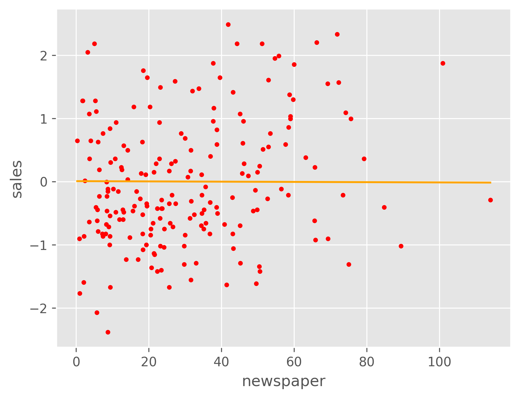
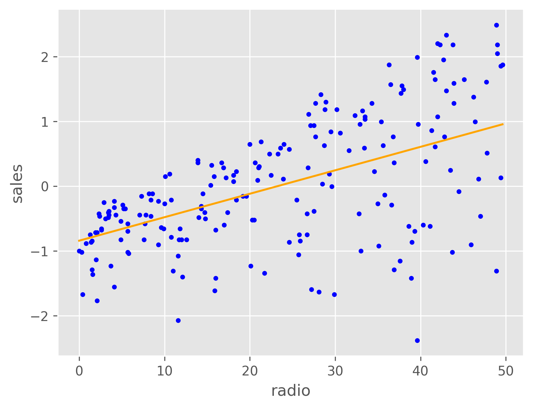
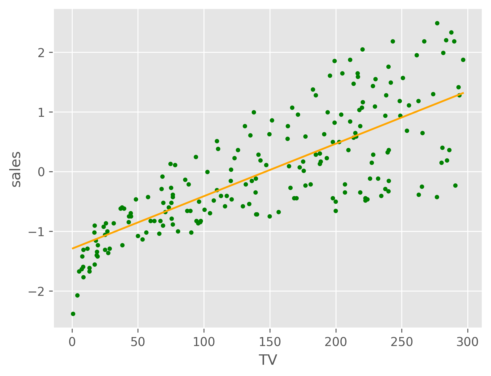
These plots show that the model fits the regression lines for both TV and radio fairly well, but not the newspaper budget due to its nonlinear relationship with the sales, as discussed above. We can project our regression model onto the TV-Radio plane to visualize how the predicted sales varies with each.

We can make a concrete prediction using our model for some sample inputs. For example, the predicted sales for TV=230.0, radio=37.0, newspaper=20.0 is: $$ h(\begin{pmatrix} 230 \\ 37 \\ 20 \end{pmatrix}) = 20.44\text{ units} $$ Where the input budgets are in thousounds of dollars and the output in thousands of units.