A Linear Regression Analysis of Invasive Burmese Pythons
Demonstrating the use of linear regression to understand the relationship between the length and mass of invasive Burmese pythons in the Florida Everglades.
Introduction
Linear regression is a "statistical method used to model the relationship between a dependent variable and one or more independent variables". We explore how to implement linear regression using a machine learning approach, and apply it to a real dataset. Using a dataset on invasive Burmese pythons in Florida, we create a model to relate the length of these snakes to their mass. This analysis can help us understand the growth patterns of these pythons. It will also serve as a simple example of how regression techniques work and how they can be implemented.
Overview and Derivation of Linear Regression
We will focus on univariate linear regression, which involves a single independent variable and a single dependent variable, both of which are real numbers. We assume that there is a linear relationship between these variables, such that there is a function $h: \mathbb{R} \to \mathbb{R}$, where h has the form $h(x)=w0x+w1$. The function h is called the hypothesis function, and our goal is to find the weights w0 and w1, such that h is the straight line that fits the data as closely as possible. In order to be precise we introduce another function, called the loss function, which we use to evaluate our model.
There are several different choices for the loss function, $L: \mathbb{R} \times \mathbb{R} \to \mathbb{R}$, but we will focus on the L2 loss, which is defined as $L(y, h(x)) = (y - h(x))^2$. The L2 loss is the squared difference between the actual value y in our dataset, (e.g., mass), and the predicted value h(x), which is our model's predicted output for the input x (e.g., length). It is important to note that the loss function is a function of the weights, w0 and w1, not of x and y. The x and y come from our dataset and are treated as fixed constants in the context of the loss function. The goal is to find the w0 and w1 which minimize the total loss over all data points, which is given by the sum of the L2 losses for each data point, where n is the number of data points: $$L_{total} = \sum_{i=1}^{n} L(y_i, h(x_i)) = \sum_{i=1}^{n} (y_i - h(x_i))^2$$
Gradient Descent
To find the optimal weights w0 and w1 for our model, we can use an optimization algorithm called gradient descent. The idea is to iteratively update the weights in the direction of the negative gradient of the loss function. The negative of the gradient points in the direction of the steepest descent of a function, so by moving in this direction, the value of our L2 loss function will descrease by the largest amount at that point (w0, w1, L(w0, w1)), bringing us closed to minimum with each iteration. It should be noted that since the L2 loss is a convex function, it has a unique global minimum. The update rule for gradient descent is given by: $$w_j := w_j - \alpha \cdot \frac{\partial L_{total}}{\partial w_j}$$ where $\alpha$ is the learning rate, which controls how much we adjust the weights at each step. The gradient of the total loss in this case is given by: $$ \nabla{}L_{total} = \begin{Bmatrix} \frac{\partial L_{total}}{\partial w_0} \\ \frac{\partial L_{total}}{\partial w_1} \end{Bmatrix} = \begin{Bmatrix} -2 \sum_{i=1}^{n} (y_i - h(x_i)) \\ -2 \sum_{i=1}^{n} (y_i - h(x_i))x_i \end{Bmatrix} $$
Dataset
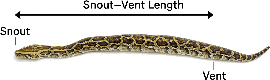
For this analysis, we will use a dataset of invasive Burmese pythons captured in the Florida Everglades. The dataset was obtained from the USGS and contains length, total mass, fat mass, and specimen condition data for 248 Burmese pythons (Python bivittatus) collected in the Florida Everglades [1]. While it is a relatively small dataset, it is perfect for our purposes. We will focus on the length and mass attributes from the dataset to train our regression model, where the length is the SVL, or snout-vent length, given in cm, and the mass is the total mass of the python in grams.
Results
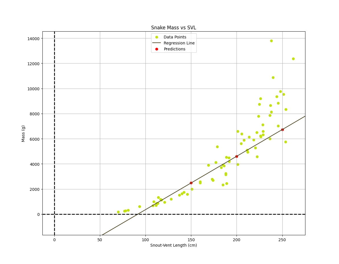
Using gradient descent to create our linear regression model, we can visualize the data points to see the relationship between length and mass. The resulting line will give us the predicted mass for a given length of python. We can also calculate the coefficients w1 and w0, which represent the slope and intercept of the line, respectively.
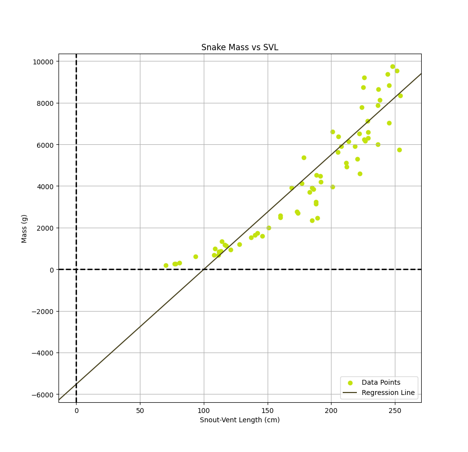
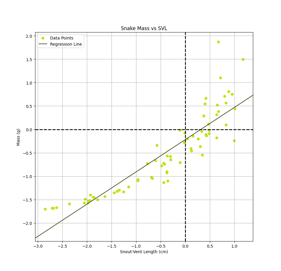
The final linear model, in units of grams for the mass and cm for the svl, is: $$h(x) = mass(svl) \approx 55.11svl -5519.45$$ In order to speed up the convergence of gradient descent and obtain these final weights, it was necessary to standardize the data by subtracting the mean, $\mu$, and divide by the standard deviation, $\sigma$, so the data we use to the train the model is $ svl_{scaled} = \frac{svl - \mu_{svl}}{\sigma_{svl}} $ and $ mass_{scaled} = \frac{mass - \mu_{mass}}{\sigma_{mass}} $. We can then obtain the weights in the correct scale by performing an appropriate transformation back to the original units. The standardized model is shown below as well as an animation depecting how the regression line changes during the training process. $$h(x) = mass(svl) \approx 0.6893svl -0.2195$$
Using our model we can make some concrete predictions of the mass of a Burmese python of a given length found in the Florida Everglades. For example, our model predicts: $$ \begin{align*} mass(150cm) \approx 2481.84g \\ mass(200cm) \approx 4605.91g \\ mass(250cm) \approx 6729.99g \end{align*}$$
Conclusions
We have successfully applied linear regression to analyze the relationship between the length and mass of invasive Burmese pythons in the Florida Everglades. The results show that there is a positive correlation between the two variables, indicating that as the length of the python increases, so does its mass. In particular, the weight w1 representing the slope, indicates that for each cm increase in svl of a python, the mass increases by about 55.11 g. The intercept of the regression equation, given by w0, technically estimates the mass of a python with zero snout-vent length. While a snake with no length would have no mass, it serves as the base level from which the model's linear growth pattern extends. Given that our model predicts negative mass up until about a 100cm svl, the model's predictions are only physically meaningful for lengths larger than this.
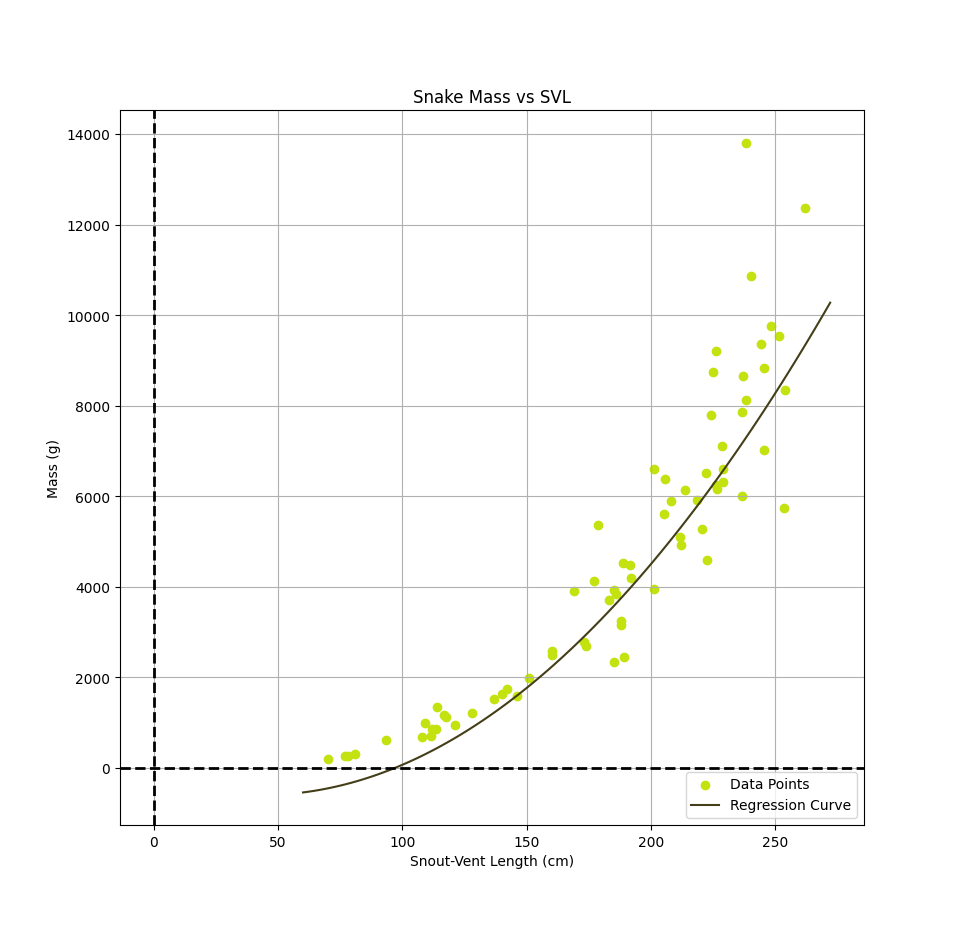
Observing the data points on the graphs, it appears as though a polynomial may be a better fit to the data. Using a related technique, polynomial regression, we fit a quadratic to the data resulting in a new model. While this was not the primary focus, the quadratic model ended up achieving a lower loss of around 7, while the linear model had a loss of around 10. This means that the squared distances between our model's predicted values and the actual values are smaller for the quadratic model than for the linear model, meaning the quadratic model produced predictions closer to the actual values in our dataset. The quadratic model is given by: $$h(x) = mass(svl) \approx w2svl^2 + w1svl - w0$$ We can train this model using the same gradient descent approach, but we now have 3 weights and the gradient of the loss function becomes: $$ \nabla{}L_{total} = \begin{Bmatrix} \frac{\partial L_{total}}{\partial w_0} \\ \frac{\partial L_{total}}{\partial w_1} \\ \frac{\partial L_{total}}{\partial w_1} \end{Bmatrix} = \begin{Bmatrix} -2 \sum_{i=1}^{n} (y_i - h(x_i)) \\ -2 \sum_{i=1}^{n} (y_i - h(x_i))x_i \\ -2 \sum_{i=1}^{n} (y_i - h(x_i))x_i^2 \end{Bmatrix} $$ This can be generalized to polynomials of higher degree, but for now we focused only on a quadratic model. The result on our Python dataset is plotted below.
The analysis could be extended by incorporating additional features of the dataset, such as fat mass or habitat, to predict the mass. We could also examine other snake species to see if our model generalizes. Another possibility would be to incorporate many different snake species into the model to see if the relationship holds across species. This would require a more complex model, such as a multivariate linear regression, but it could provide valuable insights into the growth patterns of these snakes.